


This is the first of a three-part series examining why the automated market maker model, developed for crypto-native tokens, does not transfer cleanly to tokenized real-world assets. Part I sets out how liquidity is measured and how decentralized liquidity pools function. Part II examines why real-world assets fail to meet the conditions that make these pools workable. Part III uses Fractalized’s published architecture as a case study in an alternative design.
Editorial note: this series is written for research and educational purposes. It does not constitute investment, legal or financial advice.
The Mechanics of Market Depth
A token can move between two wallets in seconds. That does not mean its owner can sell it.
This distinction is central to a common misunderstanding in real-world asset tokenization. An asset can be fractionally owned, recorded onchain, transferred continuously and integrated with smart contracts, and still be illiquid in the sense that matters to an investor trying to exit a position.
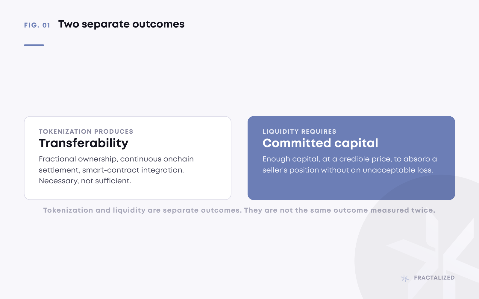
Tokenization produces transferability. Liquidity requires enough committed capital, at a credible price, to absorb a seller’s position without an unacceptable loss.
The distinction matters because much of the RWA industry has treated liquidity as an automatic byproduct of tokenization. The implicit assumption runs roughly as follows: place a building, vessel, private loan or infrastructure project onchain, issue a token, list it against a liquidity pool, and a functioning secondary market will result.
A liquidity pool does not convert an illiquid asset into cash on demand. It is a pre-funded market-making mechanism. It can buy only what its reserves permit. Its price is informative only insofar as it can be connected to the economic value of the underlying asset. Its market stays orderly only if inventory, valuation changes and adverse selling pressure are actively managed.
Recent empirical work on tokenized Treasuries, gold and private credit supports this distinction. The amount of an asset placed onchain does not reliably predict its turnover, participation or secondary-market activity. Tokenization and liquidity are separate outcomes.
This has a structural implication that runs through the rest of this series: an economically distinct real-world asset should generally have its own legal structure, its own token, its own valuation process, its own price curve and its own liquidity policy. The remainder of Part I explains why, starting from first principles of how liquidity is actually measured and how automated market makers work.
Liquidity is not a single number
Financial commentary often treats liquidity as though it were a scalar quantity: a token "has" $5 million of liquidity, a market "has" $100 million of daily volume, a protocol "has" $1 billion in total value locked.
None of these figures, on its own, tells an investor how much can actually be sold.
A more useful working definition is the ability to execute a specified trade, within a specified period, at an acceptable deviation from fair value. Liquidity is therefore a function of the size and direction of the intended transaction. A market can be highly liquid for a $1,000 order and inadequate for a $500,000 order in the same asset, at the same moment.
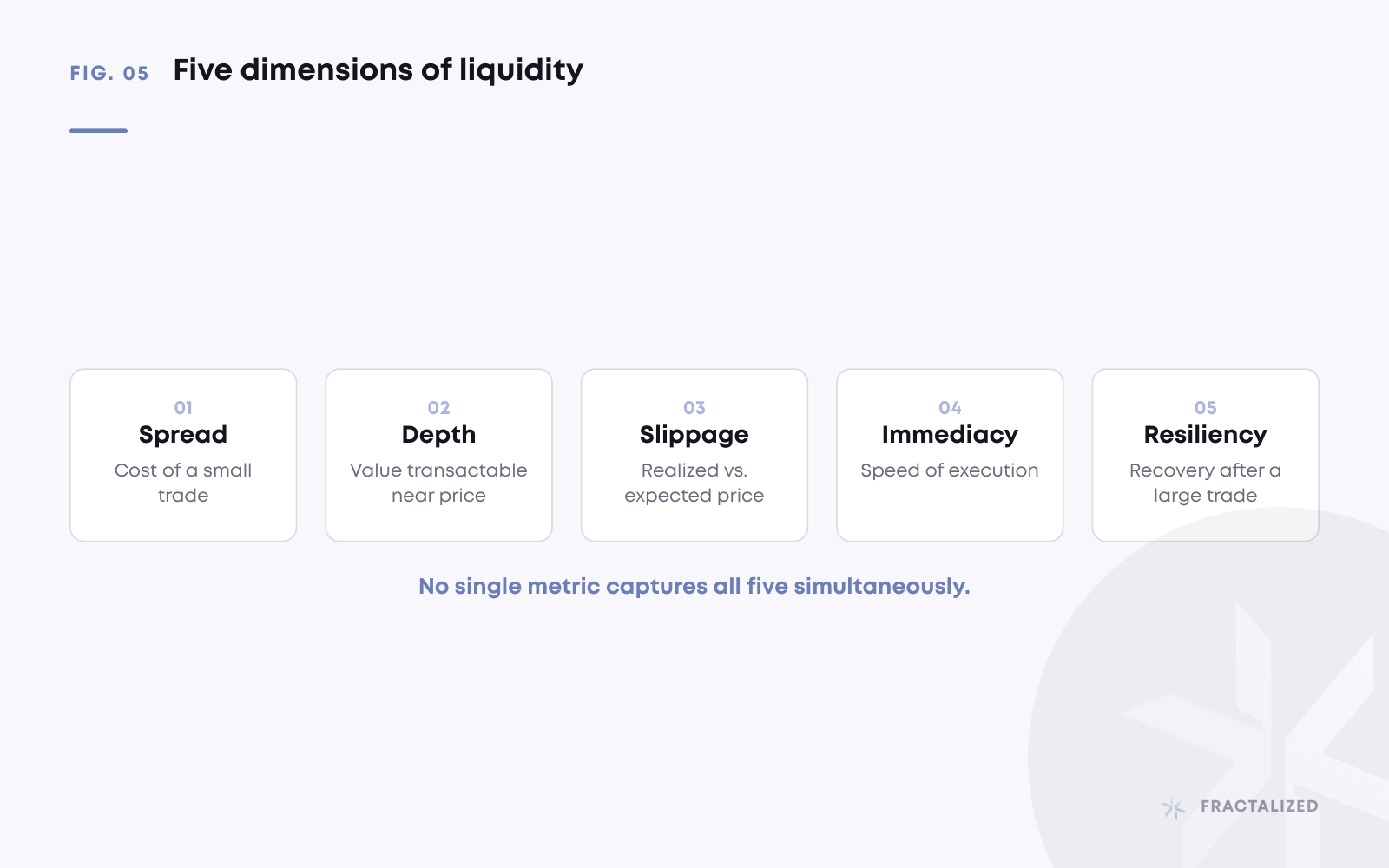
Market-microstructure research typically separates liquidity into several distinct dimensions: the cost of trading, the volume available near the current price, the price impact of a given transaction, the speed of execution, and the speed at which the market recovers after a large order. No single metric captures all of these simultaneously.
Spread
The bid-ask spread is the difference between the highest price a buyer will pay and the lowest price a seller will accept. If b denotes the best bid, a the best ask, and m the midpoint (a + b) / 2, the quoted spread in basis points is:
Spread (bps) = 10,000 × (a − b) / m
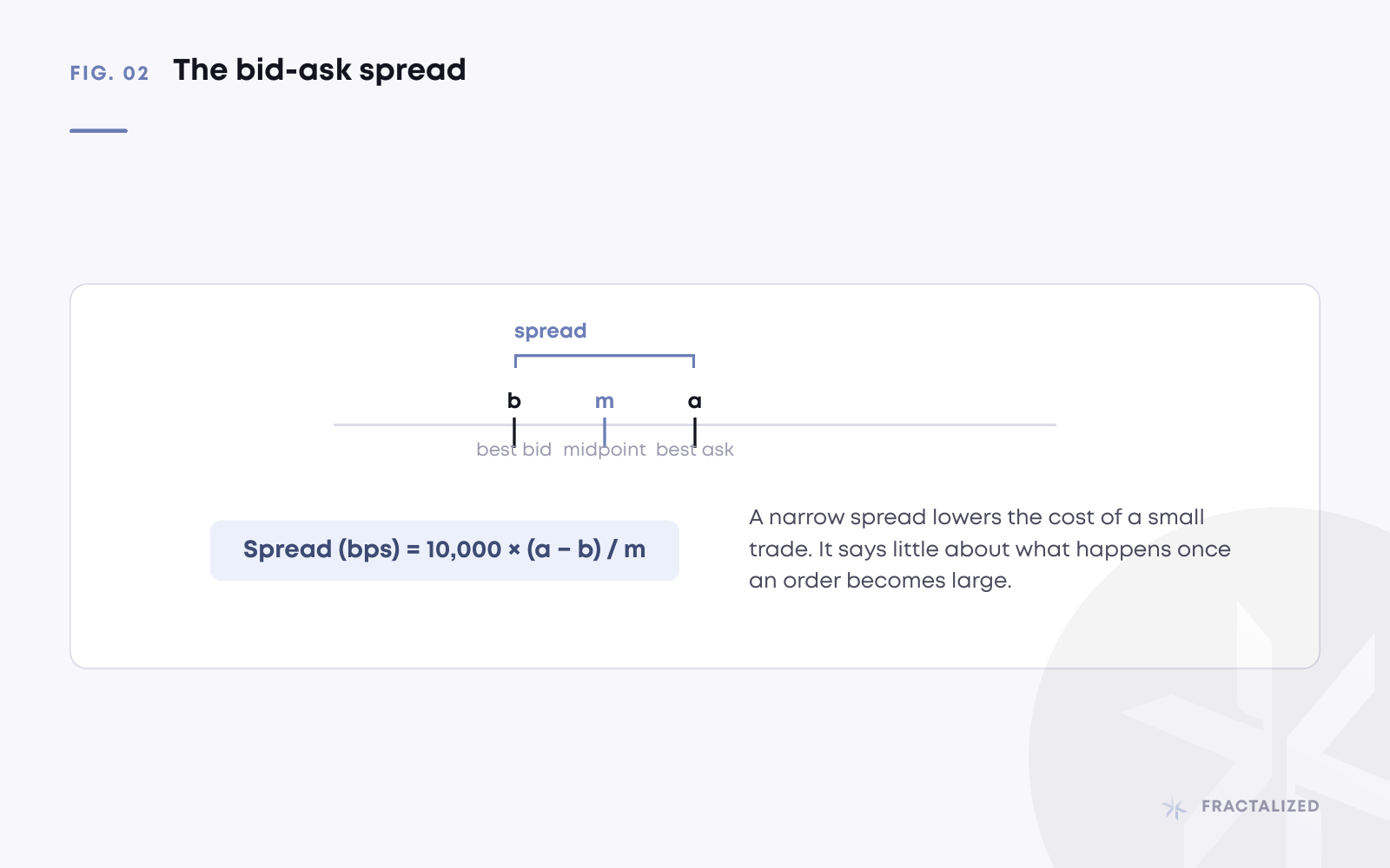
A narrow spread generally indicates that a small position can be entered and exited at low cost. It says relatively little about what happens once an order becomes large.
Depth
Depth measures how much can be transacted close to the prevailing price. A market can display a tight spread while offering only $2,000 at the best bid, with the next available buyer 5 percent lower. Under those conditions the market appears liquid until an order exceeds $2,000.
A more informative way to report depth is to disclose the dollar value available within 1, 2 and 5 percent of the reference price, along with the percentage of free-floating supply that would need to trade before those thresholds are crossed.
Slippage and price impact
Slippage is the gap between the expected price and the average price actually realized. For a buy order, slippage is the volume-weighted average execution price divided by the midpoint, less one. For a sell order, it is one minus that same ratio.
Price impact is related but focuses on how a transaction changes the market itself. The Kyle lambda, a standard measure in market-microstructure theory, estimates the price movement associated with a given amount of signed order flow. A larger lambda implies that a transaction of a given size moves the market further, which indicates lower depth.
The Amihud illiquidity measure is calculated as the average ratio of absolute price returns to dollar trading volume over a period. When modest trading volume produces a disproportionately large price movement, the measure rises. The underlying logic is straightforward: if a small amount of trading moves the price significantly, the market is comparatively illiquid.
Immediacy and resiliency
Immediacy concerns how quickly a position can be executed. Resiliency concerns what happens to the market afterward. A resilient market replenishes its bids and offers after a large trade within a short period. An unresilient market can remain dislocated for hours or days. This distinction is particularly relevant for tokenized private assets, where a single large holder may represent a substantial share of the free float.
The operative question is therefore not how much liquidity a token has in the abstract, but how much of it can be sold today, at what average price, with what price impact, and how quickly the market recovers afterward.
What a market maker actually provides
A market maker sells immediacy.
A natural buyer and a natural seller rarely arrive at the same moment with matching size. The market maker closes that timing gap by temporarily holding inventory: buying from a seller when no buyer is immediately present, and later selling to a buyer from that inventory.
Compensation for this service reflects several risks. The asset held in inventory may decline in value before it can be resold. The counterparty on the other side of a trade may possess superior information. Capital must be committed on both sides of the market simultaneously. The position may require hedging, financing, valuation and ongoing operational management.
On a centralized exchange, a professional market maker adjusts continuously to these conditions: widening spreads during periods of uncertainty, reducing bid size, cancelling stale orders, or skewing prices to encourage trades that reduce an unwanted inventory position.
An automated market maker, or AMM, performs a comparable inventory function through different means. Rather than publishing and continually revising individual bids and offers, an AMM commits deposited assets to an algorithmic price curve inside a smart contract. Any participant can trade against that curve while inventory remains available.
The design has genuine advantages: an AMM can quote continuously without a centralized intermediary and settle transactions atomically onchain. It remains, however, an inventory-holding entity exposed to informed traders, and it still requires capital to function.
How constant-product liquidity pools work
The foundational DeFi liquidity-pool design is the constant-product automated market maker, popularized by Uniswap. Its invariant is x × y = k, where x is the quantity of the first token held in the pool, y is the quantity of the paired quote asset such as USDC, and k is held constant.
The pool's marginal price for the first token, expressed in units of the second, is approximately y / x. When a participant buys the first token, its quantity in the pool falls and the USDC quantity rises, so the implied price increases. When a participant sells the token, the reverse occurs and the price falls.
The pool does not form an independent judgment about whether the token is worth more or less. It moves along a predetermined inventory curve. The label attached to the token is irrelevant to the contract: it does not distinguish a governance token, a share in a vessel, or a tokenized bond. It tracks only its own reserves and its invariant.
Why total value locked can be misleading
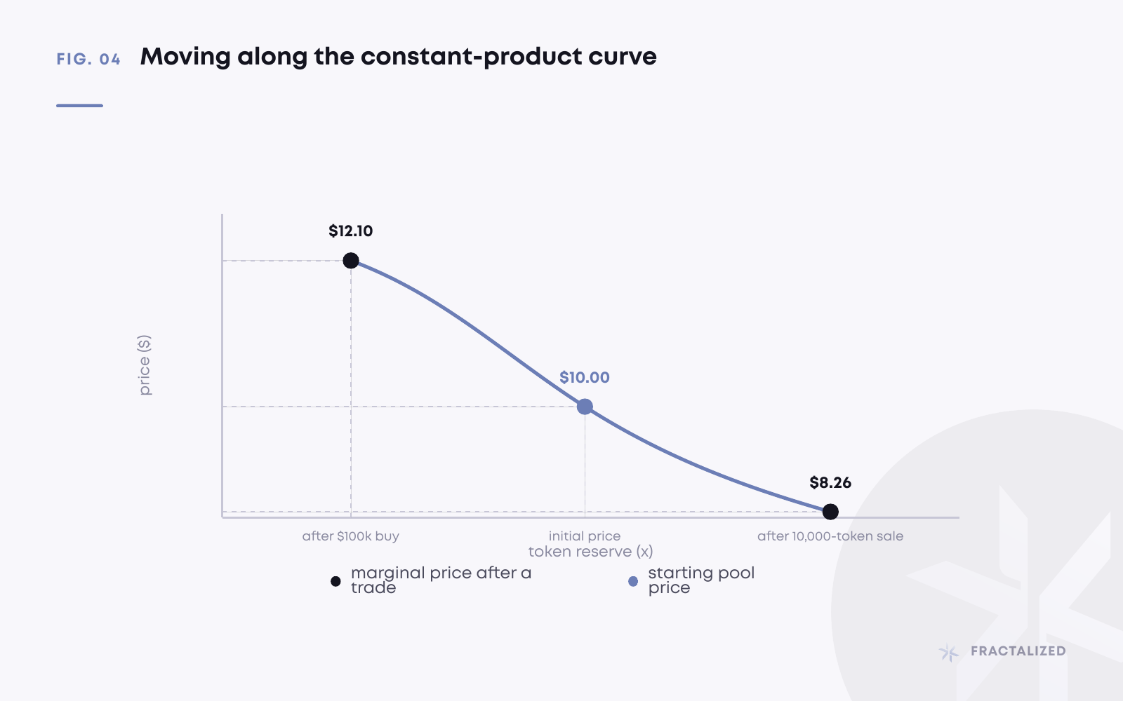
Consider a pool holding 100,000 tokens and 1,000,000 USDC. The initial price implied by the pool is 1,000,000 divided by 100,000, or $10. At that price, the pool's headline total value is $2 million, split evenly between the token and USDC.
That figure does not mean an investor can sell $1 million of the token at $10. Ignoring fees, a buyer depositing $100,000 receives approximately 9,090.91 tokens, at an average execution price of $11, with the marginal pool price rising to roughly $12.10. A seller depositing 10,000 tokens receives approximately $90,909, at an average execution price near $9.09, with the marginal price falling to roughly $8.26.
A transaction equal to 10 percent of one side of the pool produces roughly 10 percent average slippage and moves the marginal price considerably further. A headline figure of "$2 million of liquidity" is therefore an inventory valuation, not an execution guarantee. The economically relevant information is the pool's slippage curve: how the average execution price changes as order size increases.
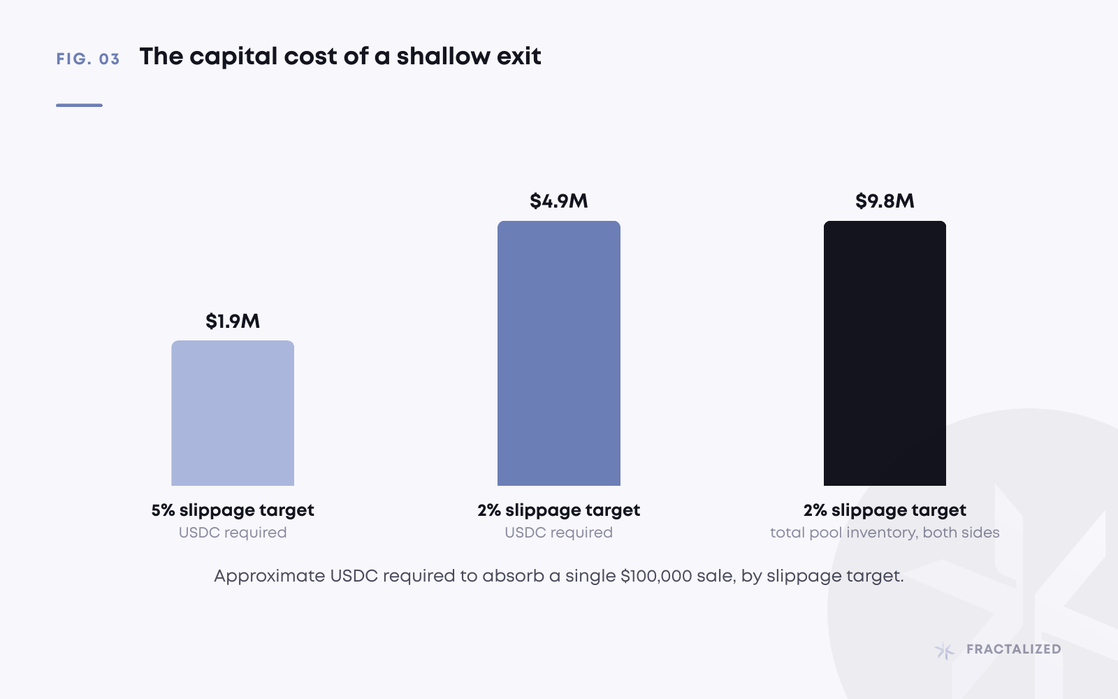
The same arithmetic indicates how much quote capital is required to support a given exit. To absorb a $100,000 sale at no more than 5 percent average slippage, a balanced constant-product pool needs approximately $1.9 million of USDC. To hold slippage to 2 percent for the same sale, it needs approximately $4.9 million. Supporting a $100,000 sale at 2 percent average slippage from a balanced full-range pool therefore requires close to $9.8 million of total inventory. This is why passive, full-range AMMs are capital intensive relative to the depth they provide.
Concentrated liquidity and its trade-offs
Uniswap v3 introduced concentrated liquidity. Rather than distributing capital across every theoretically possible price from zero to infinity, a liquidity provider selects a bounded price range and concentrates capital inside it. This produces substantially greater depth near the prevailing price and is the dominant design for volatile token pairs, because it allows capital to be used more efficiently than a full-range position.
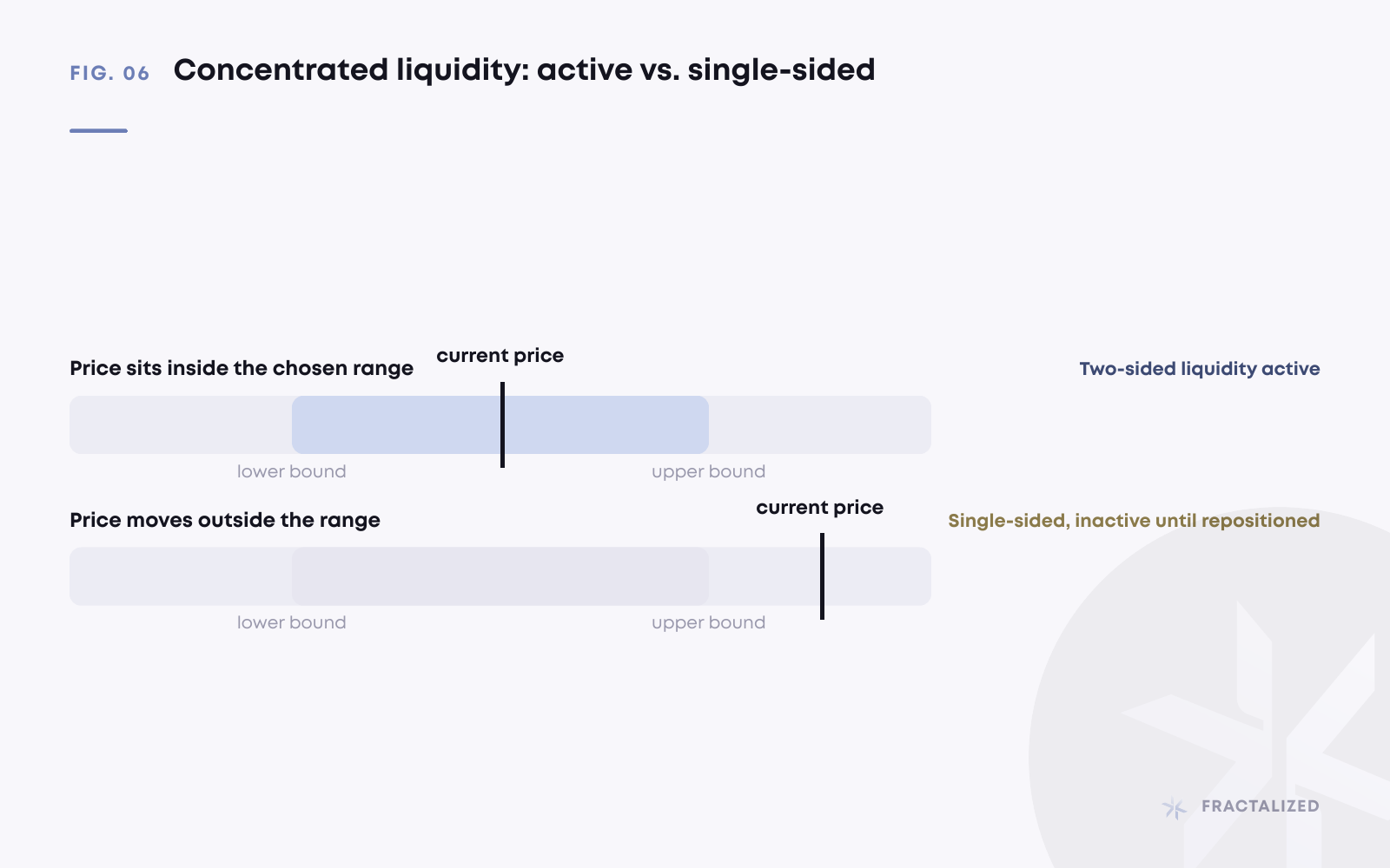
The trade-off is that once the market price moves outside the selected range, the position becomes single-sided and stops providing active two-sided liquidity. It must be repositioned to become active again. Uniswap's own documentation describes this transition explicitly: liquidity is active only inside the chosen range and converts entirely into one asset once a boundary is crossed.
Concentrated liquidity does not eliminate the need for liquidity management. It increases its importance, since someone must select the range, monitor the market, rebalance inventory, and decide what to do as price approaches a boundary.
Other AMM designs address different asset characteristics. Curve's StableSwap combines behavior resembling a constant-sum market near parity with constant-product protection further from parity, suited to assets expected to remain close in value, such as different dollar stablecoins, rather than assets with unrelated economic risk profiles. Balancer generalizes the constant-product design into weighted, multi-asset pools, which can function as self-balancing portfolios but also expose healthier assets in the pool to trading against a deteriorating one. DODO's Proactive Market Maker uses an external reference price and adjusts quotes as inventory departs from a target level, a design closer in spirit to professional market making.
The general pattern: volatile crypto pairs typically use constant-product or concentrated constant-product designs; assets expected to remain near parity use StableSwap-like curves; multi-asset portfolios use weighted invariants; and assets with a defensible reference value and material inventory risk are better served by oracle-informed or actively managed designs. Individually valued real-world assets fall much closer to the last category than the first.
Why this works for crypto-native tokens
A typical crypto-native asset has several properties that make AMM-based liquidity viable. It is usually fungible, so one unit is economically equivalent to another unit of the same token. It often trades simultaneously across multiple centralized and decentralized venues. Its market price updates continuously. It can be transferred and settled onchain without an offchain registrar, physical delivery process, appraisal, or legal title transfer. Market makers can frequently hedge exposure through other spot markets, futures, perpetual swaps or options.
These conditions support arbitrage. Suppose ETH trades at $3,000 on several large exchanges while an AMM temporarily prices it at $2,950. An arbitrageur can buy from the AMM and sell elsewhere, which removes ETH from the pool, adds quote currency, and pushes the pool price upward. If the AMM prices ETH at $3,050, the reverse trade occurs.
The pool does not discover the broader market price independently. External markets perform most of the price discovery, and arbitrageurs transmit that price into the AMM by trading against its inventory.
This creates a structural tension at the center of decentralized liquidity: arbitrage is necessary to keep the AMM aligned with the wider market, but it is costly to liquidity providers, since the arbitrageur is by definition trading against a price that has not yet adjusted. Research on loss-versus-rebalancing identifies this stale-price adverse selection as a fundamental cost of passive AMM liquidity.
Crypto AMMs remain workable in practice because the external price is visible, arbitrage can be executed quickly, the token can move across venues, settlement is largely atomic, hedging markets often exist, and trading fees together with uninformed order flow may partially offset adverse-selection costs for liquidity providers.
For many real-world assets, several of these conditions are absent.
Part II examines why, and what that absence implies for market design.